

Computed tomography lung volume estimation and its relation to lung capacities and spine deformation
Introduction
For background knowledge on idiopathic scoliosis see, e.g., the textbook (1), scoliosis is the result of a three-dimensional deformity of the vertebral column. The Cobb angle is a crude but practical measure of the deformation of the vertebral column; classification systems, such as the Lenke system, include sagittal and lumbar modifiers, variability upon bending and number of curves. A natural (but more complicated) parameter of local deformation is the (axial) apex vertebral rotation.
It is believed, in recent literature, that scoliosis can have a negative effect on lung function (2-4), regarding idiopathic scoliosis of children, where it is stated that scoliosis results in restrictive lung disease with a multifactorial decrease in lung volume. Further they state that it causes displacement of intrathoracic organs, impedes rib movement, aspects the mechanics of respiratory muscles, decreases lung compliance and results in increased work of breathing. Restrictiveness induced by scoliosis involves many factors that can simultaneously affect changes in lung function [e.g., as mentioned in (5), p. 441] and such relationship may not be strictly linear. Asymmetry of lung function could be a factor (6). It is indicated that airway compression can be caused by protrusion of an anterior vertebral body in patients with scoliosis (in relation to this phenomenon they introduce the so-called spinal penetration index) (7). It is pointed out that in patients with Cobb angle less than 60, there is seldom severe ventilator impairment or alteration of blood gases (5). It is stated that patients with a Cobb angle greater than 60 are more likely to exhibit a restrictive defect, and that in secondary kyphoscoliosis, muscle weakness is indicative of loss of vital capacity (VC), than the Cobb angle (8). Findings are presented (based upon a sample of 29 patients) that lend some support for their conjecture that neither total lung volume nor left/right lung volume ratio is affected significantly post-operatively (9). Interestingly, they use volumetric reconstruction from CT scans. On the other hand, a long-term follow-up study (10) indicates a gradual relative increase in normalized VC. Regarding the second part of this paper, it is possible to use DICOM data from, e.g., CT scans to estimate the volume of the lung. To obtain an estimate a single breath-hold for about 20 seconds can be used for the total lung volume. In 1994, lung volume was estimated via three methods, one of which was based on CT scans, and showed that CT scan estimates (as well as the other two methods they studied) of lung volume in children correlate well with the total lung volume measured from plethysmography (11). In 1998, lung volume estimations were studied using helical CT at inspiration and expiration. They compared the estimates on inspiration to the total lung capacity (TLC), and based on 72 patients with suspected pulmonary disease, they present a correlation coefficient of 0.89 (12). The technique of using CT scans for assessing lung volumes has also been applied in the study of patients deceased by drowning (13). In 2007, CT-based volumetric reconstruction was used in connection with spinal deformities (indicating that lung volume decreases with increasing rib hump and that asymmetry increases) (14). Other examples, where CT is used to estimate lung volumes (5,15,16). We mention however, that this method is not free from criticism (17).
We consider in this paper two issues with regard to scoliosis and vital capacities. The method and results of these two objectives are presented with some distinction, using the notation Part I and II, respectively.
The specific aim of Part I was to investigate if a linear relationship exists between normalized VC (or TLC) and apex rotation or Cobb angle respectively, and, if not, to investigate whether we can find a subdivision with respect to apex rotation (or Cobb angle) such that the subgroups differ significantly with respect to the mean of the stochastic variable associated with the sample mean of VC (or TLC), of the subgroup (note that finding subgroups such that the groups with higher spine curvature have lower VC does not advocate for a linear relationship). The aim of Part II was to investigate a method where medical imaging is used to estimate the TLC or VC, from a chest CT. This should be done such that the estimates correlate well with the normalized spirometry/plethysmography. Clinically it is of interest to verify the effect of spine deformation and selected lung volumes. Also as a side note, in most cases, preoperative idiopathic scoliosis patients are very young and in some cases it is not uncomplicated to follow the instructions for performing a spirometry adequately. This may also be a problem in the case of a diagnosis that causes cognitive impairment for example. In such cases, even crude estimates of lung volumes from CT may be of value.
Methods
The inclusion criteria were consecutive patients for whom surgery was planned and who underwent preoperative low-dose chest CT and preoperative spirometry/plethysmography. The patients all had a thoracic scoliosis curve (but it need not be the primary curve, i.e., we did not exclude patients who also had, a possibly larger, lumbar scoliosis curve), predominantly right convex. The number of patients in Part I was 63; 59 of which had idiopathic scoliosis (the predominant type) and 4 had neuromuscular scoliosis. In Part II, the number of patients was 61. The patient groups of the two parts had some mutually exclusive members, because for some patients we had access to spirometry (and in the case of TLC, plethysmography) values but the patients’ CT was not compatible with our software and vice versa. No patient had any additional severe (non-asthmatic) diagnosis affecting lung function.
Scanning device details
All chest CT were preoperative. The scanning device was, SOMATOM Definition Flash, Siemens Medical Solutions, Forchheim, Germany. The CT used 4 mm intervals. The associated software for analyzing DICOM, was Sectra, IDS7, including the application MPR.
Normalization of VC and TLC was made to previous work of Hedenström et al. (18,19) which takes into account gender, age, height and smoking.
Part I
Figure 1 presents the group divisions with respect to apex rotation and Cobb angle respectively. The intervals corresponding to each group are not evenly distributed and this modification was made mainly in order to obtain better statistics. The group of patients with the largest Cobb angles is rather small because the fact that such patients are relatively rare, at least in our sample patients. A division with forced fixed values of Cobb angle or apex rotation would render subgroups with severely unbalanced number of members. Indeed, this is primarily a preoperative group which means that most of the patients will have a minimum Cobb angle but simultaneously have not yet reached the severely high levels (because they are usually operated before this happens), for instance as we have written the group with highest Cobb angles would be very small if we did not adjust the lower bound.

For comparison we also performed the more simplistic analysis of subdividing into only two groups in which case we are able to dictate forced numbers of apex rotation or Cobb angle respectively and still obtain an almost balanced amount of patients in each group. In this case we used the following group subdivision.
As a measure of fitness of the linear model, we used sample correlation coefficients, denoted ρ and the coefficient of determination (denoted R2, will simply be the square of the correlation coefficient, but obviously lacking the information contained in the sign). See Supplementary for explanations of some statistical facts formulas and models used in the text.
Measuring the rotation of the apex vertebra and sacrum to table angle
The rotation of the apex vertebra was measured manually, based on the method of Aaro and Dahlborn (20), with the requirement that the chosen line in the method, passes through the vertebral groove [for alternative methods/representatives of rotation (21)]. The method for measuring the rotation can be described in the following steps:
- Find an appropriate plane in 3D, that passes through an estimation of the center of mass of the apex (see Figure 2).
- Find a line, in the plane from step (I) that passes through the neural groove (in the posterior of the spinal canal) such that the line divides the 2D slice of the vertebral body into two parts roughly symmetric with respect to mass.
- The apical rotation in the sense of Aaro-Dahlborn (with the requirement that the chosen line pass through the vertebral groove), denoted ‘Rotation A_D’ in the supplementary data sets, is then the angle between the line in step (II) and a line passing through the same neural groove as in step (II) and also passing through the exterior mid of the sternum at the level of the plane chosen in step (I) (see Figure 3). Although our choice of the direction of the line in step (II) was made manually, we have a posteriori, verified that our choice is compatible with the following type of symmetry about the neural groove: there is a circle in the plane chosen in step (I), such that the circle is centered at the neural grove in that plane, and defines precisely two points on the interior boundary of the sacral canal, such that the angle at the neural groove, defined by the three points has bisector, that coincides with our chosen line in step (II).


Part II
MIALite, medical image post-processing software, was used (22). We adopt the following notations. We assume we have n patients, and that we have the normalized VC values from spirometry/plethysmography, collected in the vector, L =(L1,…, Ln) and a measure (estimation/representation) of a parameter that reflects the normalized VC, estimated from CT, collected in the vector L’ =(L’1,…, L’n). We also use the normalized TLC collected in the vector T =(T1,…, Tn) and a measure (estimation/representation) of a parameter that reflects the normalized TLC, estimated from CT, collected in the vector T’ =(T’1,…, T’n). For simplicity, when it is clear from the context, we often denote by L and L’ (and T and T’) also the corresponding underlying variables describing the estimate of the normalized TLC (VC) from spirometry (and in the case of TLC plethysmography) and CT-parameter respectively1. Our goal was to search for evidence of a model of the form, L(L’) =α + βL’ or L’(L)=α + βL, α, β ∈ (−∞, ∞), β≠0. In the Supplementary we give some statistical explanations and motivations for such a model.
If the reader is uncomfortable with the language used in this section we suggest thinking of a simple example and drawing comparisons. For instance, if one measures the resting heart rate of 3 patients then the data can be collected in vector form x = (x1, x2, x3). So x denotes just the data vector. But it is common to abuse notation and also denote the variable ‘Resting heart rate’ by the letter x.
The two CT volume parameters explained
There is no exact counterpart in our collection of CT scans for any specific spirometry/plethysmography volume. For example, the CT-scans end at different levels apically, and in general large parts of the airways in the neck can be absent. Thus we cannot find the natural counterpart to TLC in all of our CT scans. Also, our CT scans are inspiratory, so we cannot use the difference between inspiratory and expiratory CT scans to estimate the residual volume. Furthermore, we do not know that the inspiration is given maximal effort by the patients. This makes it reasonable to exclude dead space type of volumes (e.g., large bronchii) from the CT volumetric estimation because these types of volumes will be relatively unaffected by whether or not the inspiration is maximal, whereas the lung volume will certainly be affected. We could choose an anatomic structure which will be apparent in our CT scans, and use it as an apical ‘cut-off’ in order to try to find a representative in the scans that could relate appropriately to TLC. In our paper, we denote by estimated lung volume parameter from CT, the volume obtained by removing the main larger bronchus structures from the total airways in a given CT. Hence, we have investigated two different relationships on which we have performed regression. We test: (I) VC can be modeled effectively (in an appropriate domain) as being in a linear relationship with the estimated lung volume from the CT scan (where the CT representation excludes the major bronchii). (II) TLC can be modeled effectively (in an appropriate domain) as being in a linear relationship with the volume of the airways from the CT scan, up to the peak of the lungs (relative to the vertebral column, e.g., if the uppermost part of the lungs reaches C2, we block the segmentation of airways at that level).
We then compare the two models by looking at which gives the best regression. Figure 4 displays an example of estimated lung volume according to model (a) where we try to relate it to normalized VC in a linear way.

Figure 5 displays an example of estimated lung volume according to model (b) including the volume of the airways from CT up to the vertical peak of the lungs which we in try to relate to normalized TLC in a linear way.

Results
Part I
Figure 6 shows (for the case of subdivision into three groups, according to Figure 1) the percentage increase in the mean of the normalized VC for the groups with a higher interval of representative for spinal curvature. Figure 7 presents the 95% confidence intervals (denoted by Iµ0.95%) for the underlying stochastic variables, µ, associated with the mean of the normalized VC (i.e., the variable for which the sample mean of the subgroup becomes an observation), for each of the groups and each of the subdivisions with respect to apical rotation and Cobb angle respectively (Supplementary in Part II regarding the terminology ‘stochastic variable’ and ‘observation’ respectively). Let µ11, µ12, µ13 denote the underlying stochastic variables associated with the means of the 3 subgroups respectively, with regard to the apical rotation subdivision of the original 63 patients. Let µ21, µ22, µ23 denote the underlying stochastic variables associated with the means of the 3 subgroups respectively, with regard to the Cobb angle subdivision (see Figure 1 for details on the different subgroups). Let  denote the sample mean of subgroup ij. For example
  is the mean of the vector with n11 =13 elements, where each element corresponds to the normalized VC of a patient with apical rotation between 0 and 8 degrees. Figure 6 gives the individual 95% confidence intervals for the µij. Figure 8 depicts the normalized VC for all three subgroups versus the apical rotation and Cobb angle respectively (see Figure 1 for details on the subgroup division).


As mentioned, we have for comparison also performed the analogous, but more simplistic analysis of subdiving, but into only two groups (Figure 9). Based upon the group subdivision of Figure 9, let as before µ11, µ12 denote the underlying stochastic variables associated with the means of the two subgroups respectively, with regard to the apical rotation subdivision of the original 63 patients. Let µ21, µ22 denote the underlying stochastic variables associated with the means of the two subgroups respectively, with regard to the Cobb angle subdivision. Let denote the sample mean of subgroup ij (now obviously 1≤ i, j ≤2). Figure 10 gives the results analogous to that of Figure 6, but for the case of only two subgroups, and the corresponding confidence intervals of Figure 7 are in the two-subgroup case is presented in Figure 11. Figure 12 presents correlation coefficients for investigating whether or not linear relationships are probable.


Part II
We present the linear regression obtained in terms of the estimate of normalized TLC (data collected normalized in the vector L’), as a linear function of normalized TLC from spirometry/plethysmography (data collected normalized in the vector L) and similarly for T, T’ (Figures 13-15). For the model L’ = α + βL, where α, β are the parameters to be estimated through linear regression, we obtained the following estimates (for the correlation coefficient ρ, the coefficient of determination R2 and the sum of squares of residuals, SSR),
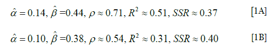
where the parameter estimates for the L, L’ model are given by Eq. [1A] and the parameter estimates for the T, T’ are given by Eq. [1B]. To test the null hypothesis H0: βL =0, for the case of L, L’ and T, T’ models respectively, and to get an idea of in what range α probably varies, we obtained the following separate 95% confidence intervals,
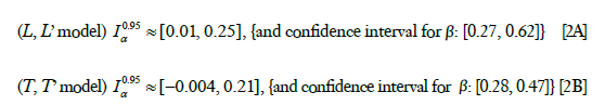
where the result for the case of L,L’ is given by Eq. [2A] and the result for the case of T,T’ is given by Eq. [2B].
We also test the hypothesis given in Part II whereby, roughly speaking2 can be identified as a constant difference between the means of L and L’. We have,


Discussion
Part I
Our results indicate (based upon a patient group of n=63 patients) that patients who fall into categories of increased (measured in terms of Cobb angle or apical rotation) severity of idiopathic scoliosis seem to have significantly reduced normalized VC (Figure 6, approximately 9% decrease of VC between adjacent groups). We have (for the case of three group subdivision) not forced specific boundary limits for the groups because that seems to render unbalanced groups (significantly different amount of members) affecting the statistical procedure negatively. On the other hand it makes sense to consider as separate groups, patients with Cobb angle close to acceptable values and patients with extremely high Cobb angles. For comparison we have, however, performed the analogous (but more simplistic) two group subdivision and for this case the results of Figure 10 gives approximately 13% decrease for the group with higher spine deformation.
Note that dividing into subgroups such that the groups with more severe scoliosis have lower VC, does not in itself indicate that a linear relationship is probable.
Figure 12 gives the correlations that have been studied in Part I. All goodness-of-fit values for investigating normalized VC or TLC versus either of apex rotation or Cobb angle respectively, are poor, and we propose, based on these values, that a linear regression model is inappropriate. But it is our belief that a, possibly analytic, relationship exists between normalized VC and each of the curvature measures but that in each case the relation is much more complicated than a mere affine relation.
We do not believe that a linear relationship is appropriate for modeling the relation between apex rotation and Cobb angle (correlation coefficient −0.53, and we do not believe the coefficient can be much improved, as little post-calculations or normalizations are used to obtain the two variables).
Clinically the results of part I do in a sense confirm (as one would expect) that the groups of severe deformity and the groups of patients that are close to being conservatively treatable respectively, differ in VC (and TLC) significantly (and they also both differ with respect to the middle group). However, we also see that the largest group in between the two extremes does not seem to vary linearly with respect to either Cobb angle or apex rotation.
Part II
Our analyses regarding the possibility of estimating of normalized TLC from inspiratory CT, suggests, based on a study of a group of patients (n=61), that a linear regression could be appropriate for describing the relationship between normalized lung volume estimated from inspiratory CT scans, and the normalized TLC from spirometry/plethysmography. The results of Figure 15, in particular the correlation coefficient of 0.71, we believe can be improved upon, see below. The analogous analysis for estimating VC shows that the latter is less appropriate.
It is customary to ask the patients to hold their breath for a few seconds and then take the scan (this is what we in this paper call an inspiratory CT scan of the thorax). However, it is not possible to know how much effort the patients have put into following the instructions to the fullest during their scans. For example, patients with large VC could have taken suboptimal breaths during their scan whereas simultaneously patients with low VC could have taken adequate breaths, leading to disruption of the hypotheses in the foundation of our model.
Many variables, such as genetics, ethnicity, dietary differences between countries, etc., are not taken into account in spirometry/plethysmography reference values. We have used reference values based on previous work of Hedenström et al. (18,19), involving gender, age, height and smoking, however the patients in that study could certainly be more focused toward our patient group. This together with the last item in the discussion, indicate possible ways of improving the correlation coefficient between normalized TLC and our CT estimates.
Conclusions
We show that a group of 63 patients (all of whom had a thoracic scoliosis curve over a wide range, possibly also a lumbar curves) could, with respect to apical rotation (or Cobb angle respectively), be divided into three subgroups, such that, pairwise, the mean of the normalized VC of the group with higher apical rotation (or Cobb angle respectively), is in some sense, at least 9% lower (in the case of two subgroups one obtains an approximate decrease of 13%). We propose that a linear regression model is inappropriate, because the correlation coefficient for the normalized VC versus apical rotation is −0.53 (and in the case of Cobb angle −0.35 respectively). The correlation coefficient between apical rotation and Cobb angles for the 63 patients was 0.64. We test a method for estimating normalized TLC from inspiratory chest CT of a group of 61 patients, all of whom had a thoracic scoliosis curve (possibly also a lumbar curve). We propose that a linear regression model could be appropriate for describing the relationship between the estimated lung volume from inspiratory CT, and the normalized TLC from spirometry/plethysmography, we obtain a correlation coefficient ≈0.71, R2 ≈0.51, although it may be possible to improve the coefficient, given more focused reference values and more stringent conditions regarding inspiration.
Supplementary
In this Supplementary appendix we gather some explanations on statistics, notations and statistical models used in the text. Recall that the correlation coefficient associated with two vectorsx=(x1,…, xn), y = (y1,…, yn), for a positive integer n, is given by,
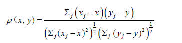
In the cases occurring in this paper the so-called coefficient of determination (often denoted, will simply be the square of the correlation coefficient, but obviously lacking the information contained in the sign of ρ).
In Part II (see Section Part II under Methods), we assume n patients, and that we have the normalized VC values from spirometry/plethysmography, collected in the vector vector L =(L1,…,Ln), and a measure (estimation/representation) of a parameter that reflects the normalized VC, estimated from CT, collected in the vector L’ =(L’1,…, L’n). We also use the normalized TLC collected in the vector T =(T1,…, Tn) and a measure (estimation/representation) of a parameter that reflects the normalized TLC, estimated from CT, collected in the vector T' =(T’1,…, T’n). We then consider a model of the form, L(L’) =α + βL’ or L’(L) =α + βL, α, β ∈ (−∞, ∞), β≠0. Such a model can also be useful even if one instead would like to study the relationship between normalized TLC and another variable, say ξ (i.e., instead of L which is our main focus), that one believes to in affine relation to the normalized VC. Namely, we could perform a linear regression of a CT parameter reflecting normalized VC (details on how this parameter is chosen are given in Section Measuring the rotation of the apex vertebra and sacrum to table angle3.2.1), 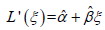 , and then use composition,
  and by being careful to use some known method on simultaneous intervals, e.g. the Bonferroni method, one could in fact estimate a confidence interval for the constants a and b; which render an affine relationship for L as a function of ξ. However, because products of estimates appear in the expressions for a and b, the confidence intervals for a and b could be quite large. One could also use the estimated intercept as a middle step by performing a t-test to (explained in layman’s layman’s terms. We use simple regression to find estimates for α and β. For comparison, we also repeated the analogous linearity analyses with L, L’ replaced by T, T’.
Data sets can be obtained from the corresponding author upon request.
Acknowledgements
The authors would like to thank the referees for their valuable comments which helped to improve the manuscript. In particular the reviewers have pointed out that if there is a second lower spine curve (by Cobb angle), it may produce pelvic obliquity that could compromise vital capacity if the iliac crest impinges on ribs on one side. The study was funded by the Swedish government in terms of ALF-grant.
Footnote
Conflicts of Interest: The authors have no conflicts of interest to declare.
Ethical Statement: The study was approved by the regional ethics committee in Linköping, Sweden (LIO-541821). The participants (or legal parent or guardian for children) have all given written consent to publish and report individual patient data.
1If the reader is uncomfortable with the language used in this section we suggest thinking of a simple example and drawing comparisons. For instance, if one measures the resting heart rate of 3 patients then the data can be collected in vector form x = (x1, x2, x3). So x denotes just the data vector. But it is common to abuse notation and also denote the variable ‘Resting heart rate’ by the letter x.
2Recall that the hypothesis is that the vectors L = (L1,…,Ln) and L’ = (L’1,…,L’n) are samples from families of normally distributed random variables with constant variance (see Supplementary), but which differ in the mean for each pair (Li–L’i), by a constant in which case the differences can be assumed to be a sample from N(µ, σ2), where  and σ2 ≥0, so we can reject at 0.95 confidence if
  .
.
3For the interested reader we point out that what one is actually doing is to test the hypothesis that the vectors L = (L1,…,Ln) and L’ = (L’1,…, L’n) are samples from families of normally distributed random variables  , with constant variance, independent of i (i =1,…,n), but which differ in mean at each i by a constant a, i.e., the null hypothesis is
  , i =1,…, n. Note that under the given hypothesis, we have i.i.d. normal distributed variables
  , so we can estimate a variance σ2 using the sample variance of the data Z = (Li–L’i,…, Ln–L’n) and use a t-test to determine if Z can be regarded as a sample from N(µ,σ2), were .
References
- Newton PO, O’Brien MF. Idiopathic scoliosis: the harms study group treatment guide. Stuttgart: Thieme, 2010.
- Koumbourlis AC. Scoliosis and the respiratory system. Paediatr Respir Rev 2006;7:152-60. [Crossref] [PubMed]
- Newton PO, Faro FD, Gollogly S, et al. Results of preoperative pulmonary function testing of adolescents with idiopathic scoliosis. A study of six hundred and thirty-one patients. J Bone Joint Surg Am 2005;87:1937-46. [Crossref] [PubMed]
- Tsiligiannis T, Grivas T. Pulmonary function in children with idiopathic scoliosis. Scoliosis 2012;7:7. [Crossref] [PubMed]
- George RB. Chest Medicine: Essentials of Pulmonary and Critical Care Medicine. Philadelphia: Lippincott William & Wilkins, 2005.
- Redding G, Song K, Inscore S, et al. Lung function asymmetry in children with congenital and infantile scoliosis. Spine J 2008;8:639-44. [Crossref] [PubMed]
- Dubousset J, Wicart P, Pomero V, et al. Spinal penetration index: new three-dimensional quantified reference for lordoscoliosis and other spinal deformities. J Orthop Sci 2003;8:41-9. [Crossref] [PubMed]
- Behera D. Textbook of pulmonary medicine. 2nd ed. New Delhi: Jaypee Brothers Medical Publishers (P) Ltd, 2005.
- Sarwahi V, Sugarman EP, Wollowick AL, et al. Scoliosis surgery in patients with adolescent idiopathic scoliosis does not alter lung volume: a three dimensional CT based study. Spine (Phila Pa 1976) 2014;39:E399-405. [Crossref] [PubMed]
- Pehrsson K, Danielsson A, Nachemson A. Pulmonary function in adolescent idiopathic scoliosis: a 25 year follow up after surgery or start of brace treatment. Thorax 2001;56:388-93. [Crossref] [PubMed]
- Schlesinger AE, White DK, Mallory GB, et al. Estimation of total lung capacity from chest radiography and chest CT in children: comparison with body plethysmography. AJR Am J Roentgenol 1995;165:151-4. [Crossref] [PubMed]
- Kauczor HU, Heussel CP, Fischer B, et al. Assessment of lung volumes using helical CT at inspiration and expiration: comparison with pulmonary function tests. AJR Am J Roentgenol 1998;171:1091-5. [Crossref] [PubMed]
- Sylvan E. CT-based measurement of lung volume and attenuation of deceased. LiTH-IMT/MI20-EX-05/410-SE. Available online: https://www.diva-portal.org/smash/get/diva2:20619/FULLTEXT01.pdf
- Adam CJ, Cargill SC, Askin GN. Computed tomographic-based volumetric reconstruction of the pulmonary system in scoliosis: trends in lung volume and lung volume asymmetry with spinal curve severity. J Pediatr Orthop 2007;27:677-81. [Crossref] [PubMed]
- Gollogly S, Smith JT, Campbell RM. Determining lung volume with three-dimensional reconstructions of CT scan data: A pilot study to evaluate the effects of expansion thoracoplasty on children with severe spinal deformities. J Pediatr Orthop 2004;24:323-8. [Crossref] [PubMed]
- O'Donnell CR, Bankier AA, Stiebellehner L, et al. Comparison of plethysmographic and helium dilution lung volumes: which is best for COPD? Chest 2010;137:1108-15. [Crossref] [PubMed]
- Stanescu DC. How to measure lung volume? Chest 2010;138:1280-1; author reply 1281-2. [Crossref] [PubMed]
- Hedenström H, Malmberg P, Agarwal K. Reference values for lung function tests in females. Regression equations with smoking variables. Bull Eur Physiopathol Respir 1985;21:551-7. [PubMed]
- Hedenström H, Malmberg P, Fridriksson HV. Reference values for lung function tests in men: regression equations with smoking variables. Ups J Med Sci 1986;91:299-310. [Crossref] [PubMed]
- Aaro S, Dahlborn M. Estimation of vertebral rotation and the spinal and rib cage deformity in scoliosis by computer tomography. Spine (Phila Pa 1976) 1981;6:460-7. [Crossref] [PubMed]
- Lam GC, Hill DL, Le LH, et al. Vertebral rotation measurement: a summary and comparison of common radiographic and CT methods. Scoliosis 2008;3:16. [Crossref] [PubMed]
- Wang C, Frimmel H, Smedby Ö. Fast level‐set based image segmentation using coherent propagation. Medical Physics 2014;41:073501. [Crossref] [PubMed]

